AUC in JAGS

Another coefficient of discrimination to assess model performance

Florencia Grattarola

Last updated on 7 June 2023 5 min read

Previously, I showed how to calculate Tjur’s R2 in JAGS to evaluate the predictive performance of a presence-absence model. In this post, I will calculate AUC.

ROC and AUC

To measure the discrimination performance of our model, we can assess the agreement between predictions ($\psi$) and actual observations ($y$), based on a series of probability thresholds.

	recorded present ($y_i = 1$)	recorded absent ($y_i = 0$)
predicted present ($\psi_i = 1$)	TP (true positive)	FP (false positive)
predicted absent ($\psi_i = 0$)	FN (false negative)	TN (true negative)

Sensitivity (or the true positive rate TPR) and specificity (or the true negative rate) — measure the proportion of sites at which the observations and the predictions agree, while the false positive rate (FPR) and the false negative rate — measure the proportion of sites at which the observations and the predictions disagree (Hanley and McNeil 1982).

Sensitivity or True Postivie Rate:
$TPR = \frac{TP}{TP + FN}$
1 - Specificity or False Positive Rate:
$FPR = \frac{FP}{FP + TN}$

Over a range of probability threshold levels, each pair of true positive and false positive values can be plotted as the y and x coordinates respectively. The series of points in the graph defines a smooth curve, which is called the relative operating characteristic (ROC) curve. The area under the ROC curve, or AUC, is thus the proportion of the total area of the unit square defined by the false positive and true positive axes.

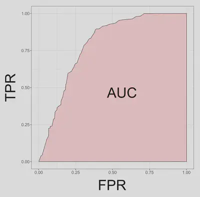
An example of ROC curve and the area under the curve (AUC). ROC curve plots TPR vs. FPR at different classification thresholds. AUC measures the area under the entire ROC curve

AUC ranges from 0.5 for models with no discrimination ability, to 1 for models with perfect discrimination. AUC between 0.5 and 0.7 indicate poor discrimination capacity, values between 0.7 and 0.9 indicate a reasonable discrimination ability appropriate for many uses, and rates higher that 0.9 indicate very good discrimination (Pearce and Ferrier 2000).

AUC Calculation

A simple way to measure the area under the ROC curve is using the trapezoidal method. For the $n$-th trapezium, the area $A_n$ is

$A_n = \frac{y_n + y_{n+1}}{2} (x_{n+1} - x_n)$

For instance, in this case,

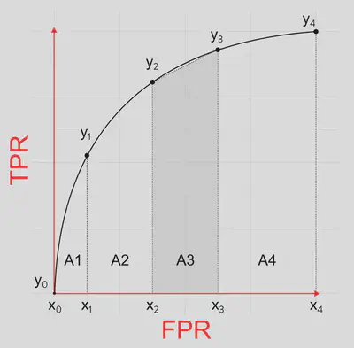
We can calculate AUC as

$A_1 = \frac{y_0 + y_1}{2} * (x_1 - x_0)$
$A_2 = \frac{y_1 + y_2}{2} * (x_2 - x_1)$
$A_3 = \frac{y_2 + y_3}{2} * (x_3 - x_2)$
$A_4 = \frac{y_3 + y_4}{2} * (x_4 - x_3)$

$AUC = A_1 + A_2 + A_3 + A_4 <= 1$

The code in JAGS will be

auc <- sum((sens[2:length(sens)]+sens[1:(length(sens)-1)])/2 * -(fpr[2:length(fpr)] - fpr[1:(length(fpr)-1)]))

See more details in this post.

Code

Here I provide the code to assess the performance of a model with a binomial response using AUC. The code to simulate the data was adapted from code written by Petr Keil. The code to calculate AUC in a JAGS model was adapted from code by johnbaums.

library(spatstat)
library(sp)
library(maptools)
library(rgeos)
library(raster)
library(gstat)
#-------
library(jagsUI) # interface to JAGS
library(tidyverse)

Data simulation

# make randomness reproducible
set.seed(1234567)  

#--------------------------------------------------------------------
# Environment
size=100
env <- im(matrix(0, size, size), xrange=c(0,1), yrange=c(0,1))
xy <- expand.grid(x = env$xcol, y = env$yrow)
g.dummy <- gstat(formula=z~1, locations=~x+y, dummy=T, beta=0,
                 model=vgm(psill=0.1, range=50, model='Exp'), nmax=20)
env <- predict(g.dummy, newdata=xy, nsim=1)

sp::gridded(env) <- ~x+y
env <- as.im(raster(env))
# scale the env. variable
env <- (env - min(env))
env <- env / max(env)

#--------------------------------------------------------------------
# Parameters
alpha <- 0  # intercept of the environment-intensity relationship
beta <- 10 # slope of the environment-intensity relationship
true.params <- c(alpha = alpha, beta = beta)

#--------------------------------------------------------------------
# True point pattern
# point process intensity lambda as a function of environment
lambda <- exp(alpha + beta*env)

# sample points using inhomogeneous poisson point process
PTS <- rpoispp(lambda)
PTS.sp <- as(object=PTS, "SpatialPoints")

#--------------------------------------------------------------------
# Generate presence-absence survey locations (polygons)
# number of survey locations
N.surv <- 50

# generate the polygons
X <- rThomas(kappa = 50,  scale = 0.2, mu = 5, win=owin(xrange=c(0,1), yrange=c(0,1)))
PLS <- dirichlet(X)
PLS.sub <- PLS[sample(1:length(PLS$tiles), size=N.surv)]

# convert tesselation to sp class
PLS.sp <- as(PLS.sub, "SpatialPolygons")

# calculate area, coordinates, abundance, and incidence in each polygon
PLS.area <- gArea(PLS.sp, byid=T)
PLS.coords <- data.frame(coordinates(PLS.sp))

names(PLS.coords) <- c("X","Y")
PLS.abund <- unlist(lapply(X = over(PLS.sp, PTS.sp, returnList = TRUE), FUN = length))
PLS.y <- 1*(PLS.abund > 0)
y <- unname(PLS.y)

thr <- seq(0, 1, 0.05)

# extract environmental variables
PLS.env <- raster::extract(x = raster(env), y = PLS.sp, fun = mean)[,1]

jags.data <- list(n = N.surv,
                  y = y,
                  area = unname(PLS.area),
                  env = PLS.env,
                  thr = thr)

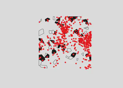
plot(PLS.sp, col = jags.data$y)
plot(PTS.sp, add=T, pch = 19, col = "red")

Model

cat('model
  {
    # PRIORS --------------------------------------------------

    ## Effect of sampling effort in PA data
    alpha ~ dnorm(0, 0.01)
    beta ~ dnorm(0, 0.01)

    # LIKELIHOOD --------------------------------------------------

    for (i in 1:n)
    {
        # the probability of presence
        cloglog(psi[i]) <- alpha + beta*env[i] + log(area[i])

        # presences and absences come from a Bernoulli distribution
        y[i] ~ dbern(psi[i])    
    }

    # POSTERIOR PREDICTIVE CHECK  --------------------------------

    # Number of recorded presences and absences
    pres.n <- sum(y[] > 0)
    absc.n <- sum(y[] == 0)

    # Sensitivity, specificity and false positive rate (1-specificity)
    for (t in 1:length(thr)) {
        sens[t] <- sum((psi > thr[t]) && (y==1))/pres.n
        spec[t] <- sum((psi < thr[t]) && (y==0))/absc.n   
        fpr[t] <- 1 - spec[t]
    }

    # AUC
    auc <- sum((sens[2:length(sens)]+sens[1:(length(sens)-1)])/2 *
    -(fpr[2:length(fpr)] - fpr[1:(length(fpr)-1)]))

  }
', file = 'auc-jags.txt')

Run

fitted.model <- jagsUI::jags(data=jags.data,
                             model.file='auc-jags.txt',
                             parameters.to.save=c('alpha', 'beta', 'psi',
                                                  'sens', 'fpr', 'auc'),
                             n.chains=3,
                             n.iter=20000,
                             n.thin=1,
                             n.burnin=2000,
                             parallel=TRUE,
                             DIC = FALSE)


Processing function input.......

Done.

Beginning parallel processing using 3 cores. Console output will be suppressed.

Parallel processing completed.

Calculating statistics.......

Done.

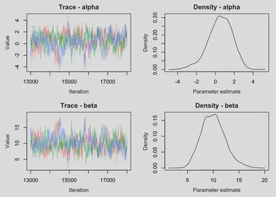
Checks

MCMCvis::MCMCtrace(object = fitted.model, params = c('alpha', 'beta'), pdf = FALSE)

# AUC
auc.sens.fpr <- bind_cols(sens=fitted.model$mean$sens,
                          fpr=fitted.model$mean$fpr)

auc.value <- fitted.model$mean$auc

auc.plot <- ggplot(auc.sens.fpr, aes(fpr, sens)) +
  geom_line() + geom_point() + coord_equal() +
  labs(x='1 - Specificity', y='Sensitivity') +
  annotate(geom="text", x=0.5, y=0.5,
           label=paste('AUC = ', round(auc.value, 3))) +
  theme_bw()

auc.plot

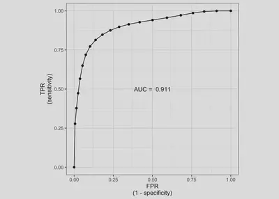
fitted.model$mean$auc

[1] 0.9113363

The results for the Tjur’s R2 for the same model simulation was 0.438.

R SDMs